Python Walkthrough

This chapter walks through using the MSG Python interface to evaluate spectra and photometric colors for a model of Sirius A (\(\alpha\) Canis Majoris A). The code fragments are presented as a sequence of Jupyter notebook cells, but pasting all of the fragments into a Python script should work also.

Preparation

Before starting Jupyter, ensure that recent versions of the NumPy, Matplotlib and Astropy packages are installed on your system. Also, make sure that the MSG_DIR environment variable is set as described in the Quick Start chapter.

Importing the PyMSG Module

Launch Jupyter, create a new Python3 notebook, and initialize the notebook with the following statements:

# Import standard modules

import sys
import os
import numpy as np
import astropy.constants as con
import astropy.units as unt
import matplotlib.pyplot as plt

# Set paths & import pymsg

MSG_DIR = os.environ['MSG_DIR']

sys.path.insert(0, os.path.join(MSG_DIR, 'python'))
import pymsg

# Set plot parameters

%matplotlib inline
plt.rcParams.update({'font.size': 16})

The sys.path.insert statement adds the directory $MSG_DIR/python to the search path, allowing Python to find and import the pymsg module. This module provides the Python interface to MSG.

Loading & Inspecting the Demo Grid

For demonstration purposes MSG includes a low-resolution specgrid (spectroscopic grid) file, $MSG_DIR/data/grids/sg-demo.h51. Load this demo grid into memory2 by creating a new pymsg.SpecGrid object:

# Load the SpecGrid

GRID_DIR = os.path.join(MSG_DIR, 'data', 'grids')

specgrid_file_name = os.path.join(GRID_DIR, 'sg-demo.h5')

specgrid = pymsg.SpecGrid(specgrid_file_name)

This object has a number of (read-only) properties that inform us about the parameter space spanned by the grid:

# Inspect grid parameters

print('Grid parameters:')

for label in specgrid.axis_labels:
    print(f'  {label} [{specgrid.axis_x_min[label]} -> {specgrid.axis_x_max[label]}]')

print(f'  lam [{specgrid.lam_min} -> {specgrid.lam_max}]')

Grid parameters:
  Teff [3500.0 -> 50000.0]
  log(g) [0.0 -> 5.0]
  lam [2999.9999999999977 -> 9003.490078514782]

Here, Teff and log(g) correspond (respectively) to the \(\Teff/\kelvin\) and \(\log_{10}(g/\cm\,\second^{-2})\) atmosphere parameters, while lam is wavelength \(\lambda/\angstrom\).

Plotting the Flux

With the grid loaded, let’s evaluate and plot a flux spectrum for Sirius A. First, store the atmospheric parameters for the star in a dict:

# Set atmospheric parameters dict from Sirius A's fundamental parameters

M = 2.02 *con.M_sun
R = 1.711 * con.R_sun
L = 25.4 * con.L_sun

Teff = (L/(4*np.pi*R**2*con.sigma_sb))**0.25/unt.K
logg = np.log10(con.G*M/R**2/(unt.cm/unt.s**2))

x = {'Teff': Teff, 'log(g)': logg}

print(Teff,np.log10(Teff))

9906.266444160501 3.9959100048166833

(the mass, radius and luminosity data are taken from Liebert et al., 2005). Then set up a uniformly-spaced wavelength abcissa for a spectrum spanning the visible range, \(3\,000\,\angstrom\) to \(7\,000\,\angstrom\).

# Set up the wavelength abscissa

lam_min = 3000.
lam_max = 7000.

lam = np.linspace(lam_min, lam_max, 501)

lam_c = 0.5*(lam[1:] + lam[:-1])

Here, the array lam defines the boundaries of 500 wavelength bins \(\{\lambda_{i},\lambda_{i+1}\}\) (\(i=1,\ldots,500\)) and the array lam_c stores the central wavelength of each bin.

With all our parameters defined, evaluate the flux spectrum using a call to the pymsg.SpecGrid.flux() method, and then plot it:

# Evaluate the flux

F_lam = specgrid.flux(x, lam)

# Plot

plt.figure(figsize=[8,8])
plt.plot(lam_c, F_lam)

plt.xlabel(r'$\lambda ({\AA})$')
plt.ylabel(r'$F_{\lambda}\ ({\rm erg\,cm^{-2}\,s^{-1}}\,\AA^{-1})$')

x_vec, deriv_vec [9.90626644e+03 4.27691898e+00] [0 0]

Text(0, 0.5, '$F_{\\lambda}\\ ({\\rm erg\\,cm^{-2}\\,s^{-1}}\\,\\AA^{-1})$')

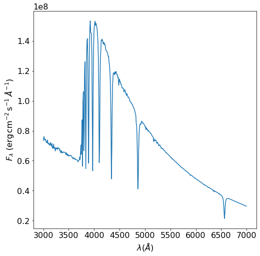
This looks about right — we can clearly see the Balmer series, starting with H\(\alpha\) at \(6563\,\angstrom\).

Plotting the Intensity

Sometimes we want to know the specific intensity of the radiation emerging from a star’s atmosphere; an example might be when we’re modeling eclipse or transit phenomena, which requires detailed knowlege of the stellar-surface radiation field. For this, we can use the pymsg.SpecGrid.intensity() method.

Here’s a demonstration of this method in action, plotting the specific intensity across the H\(\alpha\) line profile for ten different values of the emergence direction cosine \(\mu=0.1,0.2,\ldots,1.0\).

# Set up the wavelength abscissa

lam_min = 6300.
lam_max = 6800.

lam = np.linspace(lam_min, lam_max, 100)

lam_c = 0.5*(lam[1:] + lam[:-1])

# Loop over mu

plt.figure(figsize=[8,8])

for mu in np.linspace(1.0, 0.1, 10):

    # Evaluate the intensity

    I_lam = specgrid.intensity(x, mu, lam)

    # Plot

    if mu==0.1 or mu==1.0:
        label=r'$\mu={:3.1f}$'.format(mu)
    else:
        label=None

    plt.plot(lam_c, I_lam, label=label)

plt.xlabel(r'$\lambda ({\AA})$')
plt.ylabel(r'$I_{\lambda}\ ({\rm erg\,cm^{-2}\,s^{-1}}\,\AA^{-1}\,srad^{-1})$')

plt.legend()

<matplotlib.legend.Legend at 0x7fdff01a4d00>

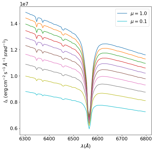
We can clearly see that limb-darkening in the line core is much weaker than in the continuum — exactly what we expect from such a strong line.

Evaluating Magnitudes & Colors

As a final step in this walkthrough, let’s evaluate the magnitude and colors of Sirius A in the Johnson photometric system. We can do this by creating a new pymsg.PhotGrid object for each passband:

# Load the PhotGrids

PASS_DIR = os.path.join(MSG_DIR, 'data', 'passbands')
filters = ['U', 'B', 'V']

photgrids = {}

for filter in filters:
    passband_file_name = os.path.join(PASS_DIR, f'pb-Generic-Johnson.{filter}-Vega.h5')
    photgrids[filter] = pymsg.PhotGrid(specgrid_file_name, passband_file_name)

(for convenience, we store the pymsg.PhotGrid objects in a dict, keyed by filter name). In the calls to the object constructor pymsg.PhotGrid(), the first argument is the name of a specgrid file (i.e., the demo grid), and the second argument is the name of a passband definition file; a limited set of these files is provided in the $MSG_DIR/data/passbands subdirectory 3. The normalized surface fluxes of Sirius A are then be found using the pymsg.PhotGrid.flux() method:

# Evaluate the surface fluxes (each normalized to the passband
# zero-point flux)

F_surf = {}

for filter in filters:
    F_surf[filter] = photgrids[filter].flux(x)

To convert these into apparent magnitudes, we first dilute them to Earth fluxes using the inverse-square law with a parallax from Perryman et al. (1997), and then apply Pogson’s logarithmic formula:

# Set the distance to Sirius A

p = 0.379
d = 1/p * con.pc

# Evaluate the Earth fluxes

F = {}

for filter in filters:
    F[filter] = F_surf[filter]*R**2/d**2

# Evaluate apparent magnitudes and print out magnitude & colors

mags = {}

for filter in filters:
    mags[filter] = -2.5*np.log10(F[filter])

print(f"V={mags['V']}, U-B={mags['U']-mags['B']}, B-V={mags['B']-mags['V']}")

V=-1.4472632983389206, U-B=-0.05922507470947869, B-V=0.0012697568194013353

Reassuringly, the resulting values are within 10 mmag of Sirius A’s apparent V-band magnitude and colors (as given by the star’s Simbad entry).

Footnotes

1

Larger grids can be downloaded separately from MSG; see the Grid Files appendix.

2

Behind the scenes, the specgrid data is loaded on demand; see the Memory Management section for further details.

3

Passband definition files for other instruments/photometric systems can be downloaded separately from MSG; see the Passband Files appendix.