Python Walkthrough
This section walks through using the MSG Python interface
to evaluate spectra and photometric colors for a model of Sirius A. The code fragments are presented as a
sequence of Jupyter notebook cells, but pasting all of them
into a Python script should work also. Alternatively, the entire notebook (including this text) is available in the source distribution at $MSG_DIR/docs/source/user-guide/walkthroughs/python-walkthrough.ipynb.
Preparation
Before starting Jupyter, make sure that you have installed the pymsg package as described in the Quick Start and/or Installation chapters. Also, ensure that the NumPy, Matplotlib and
Astropy packages are installed on your
system. Finally, confirm that the MSG_DIR environment
variable is set.
Initialization
Launch Jupyter, create a new Python3 notebook, and initialize the notebook with the following statements:
[1]:
# Import standard modules

import os
import numpy as np
import matplotlib.pyplot as plt
import astropy.constants as con

# Import pymsg

import pymsg

# Set constants

M_SUN = con.M_sun.cgs.value
R_SUN = con.R_sun.cgs.value
L_SUN = con.L_sun.cgs.value
PC = con.pc.cgs.value

G = con.G.cgs.value
C = con.c.cgs.value
SIGMA = con.sigma_sb.cgs.value

# Set plot parameters

plt.rcParams.update({'font.size': 12})
Loading & Inspecting the Demo Grid
For demonstration purposes MSG includes a low-resolution specgrid (spectroscopic grid) file, $MSG_DIR/data/grids/sg-demo.h5[1]. Load this demo grid into memory[2] by creating a
new pymsg.SpecGrid object:
[2]:
# Create the SpecGrid object

MSG_DIR = os.environ['MSG_DIR']
GRID_DIR = os.path.join(MSG_DIR, 'data', 'grids')

specgrid_file_name = os.path.join(GRID_DIR, 'sg-demo.h5')

specgrid = pymsg.SpecGrid(specgrid_file_name)
This object has a number of (read-only) properties that inform us about the parameter space spanned by the grid:
[3]:
# Inspect grid parameters

print('Grid parameters:')

for label in specgrid.axis_labels:
    print(f'  {label} [{specgrid.axis_x_min[label]} -> {specgrid.axis_x_max[label]}]')

print(f'  lam [{specgrid.lam_min} -> {specgrid.lam_max}]')
Grid parameters:
  Teff [3500.0 -> 49000.0]
  log(g) [0.0 -> 5.0]
  lam [2999.9999999999977 -> 9003.490078514782]
Here, Teff and log(g) correspond (respectively) to the
\(\Teff/\kelvin\) and \(\log_{10}(g/\cm\,\second^{-2})\) photospheric parameters, while
lam is wavelength \(\lambda/\angstrom\).
Plotting the Flux
Let’s now evaluate and plot a flux spectrum (more precisely, an irradiance spectrum) for Sirius A. First, set up the star’s parameters:
[4]:
# Set Sirius A's fundamental parameters. Mass, radius & luminosity are from
# Liebert et al. (2005, ApJ, 630, 69), while parallax and radial velocity are from
# Simbad

M = 2.02*M_SUN
R = 1.71*R_SUN
L = 25.4*L_SUN

p = 0.379
v = -5.50e5

d = 1/p * PC
z = v/C

# Store photospheric parameters in a dict

Teff = ((L/(4*np.pi*R**2*SIGMA))**0.25)
logg = np.log10(G*M/R**2)

x = {'Teff': Teff, 'log(g)': logg}
Then create a uniformly-spaced wavelength abscissa for a spectrum spanning the visible range, \(3800\,\angstrom\) to \(7000\,\angstrom\).
[5]:
# Set up the wavelength abscissa

lam_min = 3800
lam_max = 7000

lam = np.linspace(lam_min, lam_max, 501)
lam_c = 0.5*(lam[1:] + lam[:-1])
Here, the array lam defines the boundaries of 500 wavelength bins
\(\{\lambda_{i},\lambda_{i+1}\}\) (\(i=1,\ldots,500\)), and lam_c defines the central wavelength of each bin.
With all our parameters defined, evaluate the elemental flux using a
call to the pymsg.SpecGrid.flux() method, and convert it into an irradiance using equation (8) from the MSG Fundamentals chapter:
[6]:
# Evaluate the elemental flux and irradiance

F_lam = specgrid.flux(x, z, lam)
F_lam_obs = (R/d)**2*F_lam

# Plot the irradiance spectrum

plt.figure()

plt.plot(lam_c, F_lam_obs)

plt.xlabel(r'$\lambda ({\AA})$')
plt.ylabel(r'$F^{\mathrm{obs}}_{\lambda}\ ({\rm erg\,cm^{-2}\,s^{-1}}\,\AA^{-1})$');
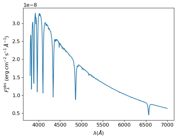
The plot looks as expected — we can clearly see the Balmer series, starting with H\(\alpha\) \(\lambda6563\,\angstrom\).
Plotting the Intensity
Sometimes we want to know the specific intensity of the radiation
emerging from an element of a star’s photosphere.
For this, we can use the pymsg.SpecGrid.intensity() method.
Here’s a demonstration of this method in action, plotting the specific intensity across the H\(\alpha\) line profile for ten different values of the angle parameter \(\mu=0.1,0.2,\ldots,1.0\).
[7]:
# Set up the wavelength abscissa

lam_min = 6300.
lam_max = 6800.

lam_H = np.linspace(lam_min, lam_max, 100)
lam_H_c = 0.5*(lam_H[1:] + lam_H[:-1])

# Loop over mu, plotting the intensity spectra

plt.figure()

for mu in np.linspace(1.0, 0.1, 10):

    # Evaluate the intensity

    I_lam = specgrid.intensity(x, mu, z, lam_H)

    if mu==0.1 or mu==1.0:
        label=r'$\mu={:3.1f}$'.format(mu)
    else:
        label=None

    plt.plot(lam_H_c, I_lam, label=label)

plt.xlabel(r'$\lambda ({\AA})$')
plt.ylabel(r'$I_{\lambda}\ ({\rm erg\,cm^{-2}\,s^{-1}}\,\AA^{-1}\,sr^{-1})$')

plt.legend();
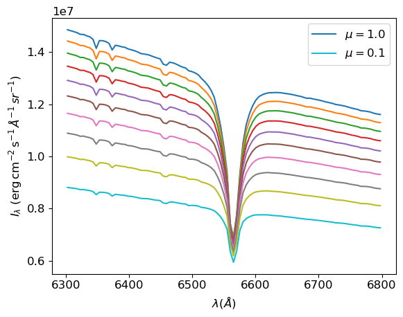
We can clearly see that limb-darkening in the line core is much weaker than in the continuum, as we exact for such a strong line.
Evaluating Magnitudes & Colors
As a final step in this walkthrough, let’s evaluate the magnitude and
colors of Sirius A in the UBV photometric system. We can do this by
creating a new pymsg.PhotGrid object for each passband:
[8]:
# Create the PhotGrid objects

PASS_DIR = os.path.join(MSG_DIR, 'data', 'passbands')
filters = ['U', 'B', 'V']

photgrids = {}

for filter in filters:
    passband_file_name = os.path.join(PASS_DIR, f'pb-Generic-Johnson.{filter}-Vega.h5')
    photgrids[filter] = pymsg.PhotGrid(specgrid_file_name, passband_file_name)
(for convenience, we store the pymsg.PhotGrid objects in a
dict, keyed by filter name). In the calls to the object constructor
pymsg.PhotGrid(), the first argument is the name of a
specgrid file (here, the demo grid), and the second argument is the
name of a passband file; a limited set of these files is
provided in the $MSG_DIR/data/passbands subdirectory[3].
The photometric irradiances of Sirius A are then found using the pymsg.PhotGrid.flux() method:
[9]:
# Evaluate the photometric irradiances (each normalized to the passband
# zero-point flux)

F_obs = {}

for filter in filters:
    F = photgrids[filter].flux(x)
    F_obs[filter] = (R/d)**2*F
To convert these into apparent magnitudes, we can apply Pogson’s logarithmic formula:
[10]:
# Evaluate apparent magnitudes and print out magnitude & colors

mags = {}

for filter in filters:
    mags[filter] = -2.5*np.log10(F_obs[filter])

print(f"V={mags['V']}, U-B={mags['U']-mags['B']}, B-V={mags['B']-mags['V']}")
V=-1.446677985580499, U-B=-0.059646818350374886, B-V=0.00112193455961207
Reassuringly, the resulting values are within 10 millimag of Sirius A’s apparent V-band magnitude and colors, as given by Simbad.
Footnotes