Line Profile Variations of a Be Star

This Cookbook recipe demonstrates how to simulate the spectral line-profile variations (lpv) of a pulsating Be star, using the MSG Python interface. The same basic approach presented in the Rotational Broadening recipe is applied here to synthesize irradiance spectra, but we must properly account for the varying photospheric parameters of the quadrature elements used in the disk integration. Calculating these parameters is beyond the scope of the recipe, and so we’ll rely on the open-source BRUCE code (Townsend, 1997) to perform the task.

Preparation

Download sg-HeI-6678.h5 and place it in your working directory (this is the same specgrid file as used in the Rotational Broadening recipe). Also download be-star-lpv.tar.bz2 and unpack it into your working directory using the tar utility. This archive contains the following items:

elements-* — quadrature element data produced by BRUCE
input.bdf — BRUCE input file used to create elements-*

Note that input.bdf isn’t needed for the recipe; it’s included for those who wish to recreate the elements-* files, or are curious about their provenance. The stellar parameters specified in input.bdf are similar to those used in the Rotational Broadening recipe, and the pulsation parameters are for a \(\ell=m=2\) mode.

Initialization

To start, import modules and set other parameters:

[1]:

# Import other modules

import numpy as np
import matplotlib as mpl
import matplotlib.pyplot as plt
import scipy.io as si
import astropy.constants as con

# Import pymsg

import pymsg

# Set constants

C = con.c.cgs.value
PC = con.pc.cgs.value

# Set plot parameters

plt.rcParams.update({'font.size': 12})

Define a Synthesis Function

Now let’s create a function that synthesizes an irradiance spectrum for a pulsating star. The synthesize_irradiance() function, defined below, takes the following arguments:

specgrid — pymsg.SpecGrid object
lam — wavelength abscissa (Å)
bruce_file — name of quadrature element file produced by BRUCE
d — distance to star (pc)

(There are significantly fewer arguments than the corresponding synthesize_irradiance() function in the Rotational Broadening recipe, because most data are provided by the BRUCE file.)

[2]:

def synthesize_irradiance(specgrid, lam, bruce_file, d):

    # Read the BRUCE file

    with si.FortranFile(bruce_file, 'r') as f:

        # Read header

        record = f.read_record('<i4', '<f4')

        n_vis = record[0][0]
        time = record[1][0]

        # Read quadrature element data, converting to cgs units

        Teff = np.empty(n_vis)
        logg = np.empty(n_vis)
        v_proj = np.empty(n_vis)
        dA_proj = np.empty(n_vis)
        mu = np.empty(n_vis)

        for i in range(n_vis):

            Teff[i], v_proj[i], dA_proj[i], g, mu[i] = f.read_reals('<f4')

            v_proj[i] *= -1e2
            dA_proj[i] *= 1e4
            logg[i] = np.log10(g) + 2

    # Evaluate dOmega (solid angle) and z (redshift)

    dOmega = dA_proj/(d*PC)**2
    z = v_proj/C

    # Set up photospheric parameters

    x = {'Teff': Teff, 'log(g)': logg}

    # Synthesize the irradiance

    F_lam_obs = specgrid.irradiance(x, mu, dOmega, z, lam)

    # Return the time and irradiance

    return time, F_lam_obs

Evaluate the Irradiance

Using the synthesize_irradiance() function, evaluate a time-series of irradiance spectra spanning the HeI \(\lambda6678\,\angstrom\) line profile:

[3]:

# Create the SpecGrid object

specgrid = pymsg.SpecGrid('sg-HeI-6678.h5')

# Set up parameters (the choice of distance is arbitrary)

d = 10

n_time = 20

# Set up the wavelength abscissa

lam = np.linspace(6670, 6690, 201)
lam_c = 0.5*(lam[:-1] + lam[1:])

# Evaluate the irradiance spectra

time = []
F_lam_obs = []

for i in range(n_time):

    bruce_file = f'elements-{i+1:03d}'

    result = synthesize_irradiance(specgrid, lam, bruce_file, d)

    time += [result[0]]
    F_lam_obs += [result[1]]

Plot the Irradiance

As a final step, plot the time-series of irradiance spectra (with an upward offset between subsequent times, to allow comparison):

[4]:

# Plot the irradiance spectra

plt.figure()

cmap = mpl.colormaps['cool']

offset=0.2*(np.max(F_lam_obs[0]) - np.min(F_lam_obs[0]))

for i in range(n_time):

    plt.plot(lam_c, F_lam_obs[i]+i*offset, color=cmap(i/(n_time-1)))

plt.xlim(6670, 6690)

plt.xlabel(r'$\lambda ({\AA})$')
plt.ylabel(r'$F^{\mathrm{obs}}_{\lambda}\ ({\rm erg\,cm^{-2}\,s^{-1}}\,\AA^{-1})$');

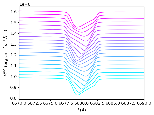
The lpv in the figure take the form of dips of enhanced absorption that travel across the line profile from blue to red. This is similar to the variations observed in pulsating Be stars (see, e.g., Štefl et al. 2003).