Light Curves of an SPB Star

This Cookbook recipe demonstrates how to synthesize light curves of a slowly pulsating B-type (SPB) star, using the MSG Python interace. The light curves are based on surface perturbation data for a \(5\,\Msun\) model, produced by the GYRE stellar oscillation code.

Preparation

Download spb-light-curve.tar.bz2 and unpack it into your working directory using the tar utility. This archive contains the following items:

• summary.h5 — surface perturbation data produced by GYRE

• pygyre — Python module for reading summary.h5

• pg-*.h5 — photgrid files for each passband[1]

• gyre.in — GYRE input file used to create summary.h5

• spb.mesa — stellar model file used to create summary.h5[2]

Note that gyre.in and spb.mesa aren’t needed for the recipe; they’re included for those who wish to recreate summary.h5, or are curious about its provenance.

Initialization

To start, import modules and set other parameters:

# Import standard modules

import numpy as np
import matplotlib.pyplot as plt
import scipy.special as ss
import astropy.constants as con

# Import pymsg and pygyre

import pymsg
import pygyre

# Set constants

SIGMA = con.sigma_sb.cgs.value

# Set plot parameters

plt.rcParams.update({'font.size': 12})

Define a Synthesis Function

Now let’s create a function that synthesizes a light curve using the semi-analytical approach described in Section 2 of Townsend (2003). The synthesize_light_curve() function, defined below, takes the following arguments:

• photgrid_file — name of photgrid file

• phi — oscillation phase array (radians)

• i — stellar inclination angle (radians)

def synthesize_light_curve(photgrid_file, phi, i):

    # Create the PhotGrid object

    photgrid = pymsg.PhotGrid(photgrid_file)

    # Read the GYRE output file into a table

    tbl = pygyre.read_output('summary.h5')

    # Select the table row corresponding to the l=m=2, g_30 mode

    mask = (tbl['l'] == 2) & (tbl['m'] == 2) & (tbl['n_pg'] == -30)

    row = tbl[mask][0]

    # Extract stellar parameters

    M_star = row['M_star']
    R_star = row['R_star']
    L_star = row['L_star']

    Teff = (L_star/(4*np.pi*SIGMA*R_star**2))**0.25
    g = con.G.cgs.value*M_star/R_star**2

    # Extract surface perturbation parameters (the T03
    # annotations indicate which equation from Townsend 2003
    # is being implemented)

    l = row['l']
    m = row['m']

    omega = row['omega']

    dR_R = row['xi_r_ref']      # Delta_R (T03, eqn. 4)
    dL_L = row['lag_L_ref']
    dT_T = 0.25*(dL_L - 2*dR_R) # Delta_T (T03, eqn. 5)
    dg_g = -(2 + omega**2)*dR_R # Delta_g (T03, eqn. 6)

    # Evaluate photometric P-moments & their partial derivatives
    # (T03, eqn. 15; the I_{l;x} in that equation is equivalent to
    # P_l here)

    x = {'Teff': Teff, 'log(g)': np.log10(g)}

    P_0 = photgrid.P_moment(x, 0)
    P_l = photgrid.P_moment(x, l)

    dP_l_dlnT = photgrid.P_moment(x, l, deriv={'Teff': True}) * Teff
    dP_l_dlng = photgrid.P_moment(x, l, deriv={'log(g)': True}) * np.log(np.exp(1.))

    # Set up differential flux functions (T03, eqns. 12-14)

    R_lm = (2+l)*(1-l) * P_l/P_0 * ss.sph_harm(m, l, 0., i)
    T_lm = dP_l_dlnT/P_0 * ss.sph_harm(m, l, 0., i)
    G_lm = dP_l_dlng/P_0 * ss.sph_harm(m, l, 0., i)

    # Construct the light curve (T03, eqn. 11)

    dF_F = ((dR_R*R_lm + dT_T*T_lm + dg_g*G_lm) * np.exp(1j*phi)).real

    # Return it

    return dF_F

Evaluate Light Curves

Using the synthesize_light_curve() function, evaluate light curves in each passband:

# Set up phase array

phi = np.linspace(0, 4*np.pi, 101)

# Set stellar inclination

i = np.radians(75)

# Evaluate light curves

dF_F_Kepler = synthesize_light_curve('pg-Kepler.h5', phi, i)
dF_F_TESS = synthesize_light_curve('pg-TESS.h5', phi, i)
dF_F_Gaia_B = synthesize_light_curve('pg-Gaia-B.h5', phi, i)
dF_F_Gaia_R = synthesize_light_curve('pg-Gaia-R.h5', phi, i)
dF_F_JWST = synthesize_light_curve('pg-JWST.h5', phi, i)

Note that the pg-JWST.h5 passband file is based on the JWST NIRCam F150W filter — chosen to demonstrate what the light curve will look like in the near infrared, but with the recognition that it’s very unlikely JWST will ever observe an SPB star!

Plot the Light Curves

As a final step, plot the light curve in each filter:

# Plot light curves

plt.figure()

plt.plot(phi/(2*np.pi), dF_F_Gaia_B, label='Gaia B', color='blue')
plt.plot(phi/(2*np.pi), dF_F_Kepler, label='Kepler', color='green')
plt.plot(phi/(2*np.pi), dF_F_TESS, label='TESS', color='yellow')
plt.plot(phi/(2*np.pi), dF_F_Gaia_R, label='Gaia R', color='orange')
plt.plot(phi/(2*np.pi), dF_F_JWST, label='JWST', color='red')

plt.xlabel('Phase (cycles)')
plt.ylabel(r'$\Delta \overline{F}^{\mathrm{obs}}\,/\,\overline{F}^{\mathrm{obs}}$')
plt.legend();

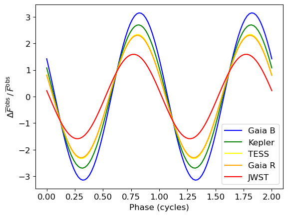
A clear trend can be seen in the light curves: from red wavelengths to blue (i.e., JWST → Gaia R → TESS → Kepler → Gaia B), the amplitude becomes larger and maximum/minimum light occur at later phases. The amplitude trend arises because the visible and NIR fall on the Rayleigh-Jeans tail of the star’s spectral energy distribution, and therefore the flux variations due to temperature perturbations vary as \(\lambda^{-4}\). The phase trend is a consequence of non-adiabatic effects that cause (for this particular mode) the radius perturbations to lag the temperature perturbations by \(\sim 45^{\circ}\).

Note that the overall scaling of the light curves is not physically meaningful; as with any linear oscillation calculation, the normalization of perturbations is arbitrary. In the case of GYRE, this normalization is chosen to yield a mode inertia of \(M R^{2}\).

Footnotes

[1]

Generated by applying the specgrid_to_photgrid tool to an extended-wavelength version of the demo grid.

[2]

Generated using the MESA stellar evolution code.