Isochrone Color-Magnitude Diagram

This Cookbook recipe demonstrates how to create a color-magnitude diagram (CMD) for an isochrone, using the MSG Python interface.

Preparation

Download isochrone-cmd.tar.bz2 and unpack it in your working directory. This archive contains the following items:

MIST.iso — isochrone data [1]
pg-*.h5 — photgrid files for each passband [2]
read_mist_models.py — Python module for reading MIST.iso

Initialization

To start, import modules and set other parameters:

[1]:

# Import modules

import numpy as np
import matplotlib.pyplot as plt

import astropy.constants as con

import pymsg
import read_mist_models

# Set plot parameters

%matplotlib inline
plt.rcParams.update({'font.size': 16})

Create PhotGrids

Next, create a pair of pymsg.PhotGrid objects for interpolating fluxes in the Johnson B and V bands:

[2]:

# Create PhotGrid objects

photgrid_B = pymsg.PhotGrid('pg-Johnson-B.h5')
photgrid_V = pymsg.PhotGrid('pg-Johnson-V.h5')

Read Isochrone Data

Now read in the isochrone data file and extract the stellar parameters:

[3]:

# Read isochrone data file

iso = read_mist_models.ISO('MIST.iso')

# Extract stellar parameters

Teff = 10**iso.isos[0]['log_Teff']
logg = iso.isos[0]['log_g']

R = 10**iso.isos[0]['log_R']*con.R_sun.value

Reading in: MIST.iso

Evaluate Fluxes

Using these parameters, evaluate the observed flux at 10 parsecs in each band:

[4]:

# Evaluate fluxes

n = len(Teff)

F_B = np.empty(n)
F_V = np.empty(n)

for i in range(n):

    # Set up photospheric parameters dict

    x = {'Teff': Teff[i],
         'log(g)': logg[i]}

    # Evaluate fluxes. Use try/execpt clause to deal with
    # points that fall outside the grid

    try:
        F_B[i] = (R[i]/(10*con.pc.value))**2 * photgrid_B.flux(x)
        F_V[i] = (R[i]/(10*con.pc.value))**2 * photgrid_V.flux(x)
    except (ValueError, LookupError):
        F_B[i] = np.NAN
        F_V[i] = np.NAN

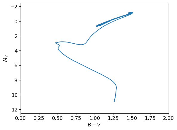
Plot the CMD

As a final step, convert fluxes to (absolute) magnitudes and plot the CMD:

[5]:

plt.figure()

M_B = -2.5*np.log10(F_B)
M_V = -2.5*np.log10(F_V)

plt.plot(M_B-M_V, M_V)

plt.xlim(0, 2)
plt.ylim(12.5,-2.5)

plt.xlabel('$B-V$')
plt.ylabel('$M_V$')

[5]:

Text(0, 0.5, '$M_V$')

../../_images/cookbook_isochrone-cmd_isochrone-cmd_9_1.png

Footnotes