Rotational Broadening

This Cookbook recipe demonstrates how to synthesize a rotationally broadened irradiance spectrum, using the MSG Python interface. At first glance, this might seem to be a trivial task: simply convolve a non-rotating irradiance spectrum with a rotational broadening function. However, as discussed in chapter 17 of Gray (2005), such an approach rests on a number of assumptions:

• that line profiles do not change shape across the stellar surface;

• that limb darkening depends only weakly on wavelength;

• that Doppler shifts arising from the rotational velocity fields can be represented as convolutions.

While these assumptions are often reasonable, there are situations where they can lead to incorrect results. A better strategy is to use equation (6).

Preparation

Download sg-HeI-6678.h5[1] and place it in your working directory. This specgrid file spans the HeI \(\lambda6678\,\angstrom\) line that will be the focus of our irradiance calculations.

Initialization

To start, import modules and set other parameters:

# Import standard modules

import numpy as np
import matplotlib.pyplot as plt
import astropy.constants as con
import scipy.io as si

# Import pymsg

import pymsg

# Set constants

M_SUN = con.M_sun.cgs.value
R_SUN = con.R_sun.cgs.value
G = con.G.cgs.value
C = con.c.cgs.value
PC = con.pc.cgs.value

# Set plot parameters

plt.rcParams.update({'font.size': 12})

Define a Synthesis Function

Now let’s create a function that synthesizes an irradiance spectrum for a rotating star. Neglecting any oblateness and gravity darkening due to the rotation, the disk integral in equation (6) can expressed in polar coordinates as

(11)\[\irrad(\lambda) = \frac{R^{2}}{d^{2}} \int_{0}^{2\pi} \int_{0}^{1} \intsy(\lambda; \mu; \vx; \vproj) \, \rho \, \diff{\rho} \, \diff\phi,\]

where \(R\) is the stellar radius, \(\rho\) the radial coordinate, and \(\phi\) the angular coordinate, oriented so that the rotation axis lies along \(\cos(\phi) = 0\). The angle parameter \(\mu\) depends on disk position via

\[\mu = \cos\left[ \sin^{-1}(\rho) \right].\]

Likewise, the projected velocity \(\vproj\) (appearing here as an additional argument of the specific intensity function) depends on position via

\[\vproj = v \sin(i) \, \rho \, \sin(\phi),\]

where \(v \sin(i)\) is the projected equatorial rotation velocity of the star.

The synthesize_irradiance() function, defined below, implements equation (11) using a simple numerical quadrature scheme. It takes the following arguments:

• specgrid — pymsg.SpecGrid object

• lam — wavelength abscissa (Å)

• M — stellar mass (\(\Msun\))

• R — stellar mass (\(\Rsun\))

• Teff — stellar effective temperature (K)

• d — distance to star (pc)

• vsini — projected equatorial velocity (km/s)

• nrho — number of \(\rho\) (radial) points in quadrature

• nphi — number of \(\phi\) (angular) points in quadrature

def synthesize_irradiance(specgrid, lam, M, R, Teff, d, vsini, nrho=128, nphi=128):

    # Set up a grid of rho and phi coordinates for the quadrature

    drho = 1/nrho
    dphi = 2*np.pi/nphi

    rho, phi = np.meshgrid(np.linspace(drho/2, 1-drho/2, nrho),
                           np.linspace(dphi/2, 2*np.pi-dphi/2, nphi))

    # Evaluate mu (angle), dA_proj (projected area) and
    # v_proj (projected velocity)

    mu = np.cos(np.arcsin(rho))
    dA_proj = ((rho + drho/2)**2 - (rho - drho/2)**2)*dphi/2
    v_proj = vsini*1E5*rho*np.sin(phi)

    # Evaluate dOmega (solid angle) and z (redshift)

    dOmega = (R*R_SUN)**2/(d*PC)**2*dA_proj
    z = v_proj/C

    # Set up (uniform) photospheric parameters

    x = {'Teff': np.full(nrho*nphi, Teff),
         'log(g)': np.full(nrho*nphi, np.log10(G*M*M_SUN/(R*R_SUN)**2))}

    # Synthesize the irradiance. The .flatten() calls are because
    # MSG expects 1-D arrays

    F_obs = specgrid.irradiance(x, mu.flatten(), dOmega.flatten(), z.flatten(), lam)

    # Return the irradiance

    return F_obs

The function uses the following algorithm:

• divide the disk into a grid of nrho by nphi quadrature elements;

• evaluate angle parameters mu, projected areas dA_proj and projected velocities v_proj of the elements;

• evaluate corresponding solid angles dOmega and redshifts z (as viewed from the observer at distance d);

• pass mu, dOmega and z, together with photospheric parameters x and wavelength abscissa lam, to the pymsg.SpecGrid.irradiance() method, which sums the contribution of each element toward the irradiance.

Evaluate the Irradiance

Using the synthesize_irradiance() function, evaluate the irradiance spectrum spanning the HeI \(\lambda6678\,\angstrom\) line profile for a B2 main-sequence star:

# Create the SpecGrid object

specgrid = pymsg.SpecGrid('sg-HeI-6678.h5')

# Set up parameters (mass, radius and effective temperature from Wikipedia,
# https://en.wikipedia.org/wiki/B-type_main-sequence_star; the choices of
# vsini and distance are arbitrary)

M = 7.30
R = 4.06
Teff = 20600.
vsini = 100
d = 10

# Set up the wavelength abscissa

lam = np.linspace(6670, 6690, 201)
lam_c = 0.5*(lam[:-1] + lam[1:])

# Evaluate the irradiance spectrum

F_obs = synthesize_irradiance(specgrid, lam, M, R, Teff, d, vsini)

Plot the Irradiance

As a final step, plot the irradiance spectrum:

# Plot the irradiance spectrum

plt.figure()

plt.plot(lam_c, F_obs)
plt.xlim(6670, 6690)

plt.xlabel(r'$\lambda ({\AA})$')
plt.ylabel(r'$F^{\mathrm{obs}}_{\lambda}\ ({\rm erg\,cm^{-2}\,s^{-1}}\,\AA^{-1})$');

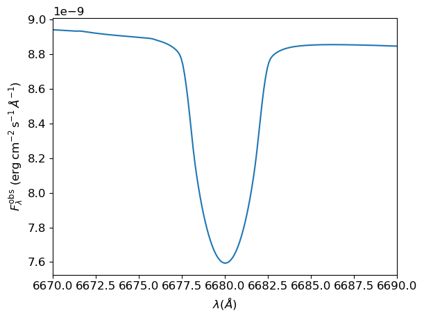
This figure shows the characteristically rounded shape due to rotation broadening. Note that the line center is around \(6680\,\angstrom\), rather than \(6678\,\angstrom\), because the sg-HeI-6678.h5 grid adopts vacuum rather than air wavelengths.

Footnotes

[1]

Generated by applying the subset_specgrid tool to the high-resolution BSTAR2006 grid.