Data Caching

This chapter discusses MSG’s data caching, a key component of its performance and scaleability. Each instance of a grid data type (e.g., specgrid_t in Fortran, or pymsg.PhotGrid in Python) has an associated cache that temporarily stores spectroscopic and/or photometric data for use in interpolations. This grid cache is initially empty when the instance is created, but grows in size as data are loaded on-demand from disk. Eventually, once a user-definable size limit is reached, old data are discarded from the cache to make room for new.

Caching Demo

With its caching functionality, MSG can in principle work with grids that are much larger on disk than available computer memory. The following Python code fragments showcase this capability, while also illustrating the basics of inspecting and controlling a grid cache.

To get started, download the sg-CAP18-coarse.h5 spectroscopic grid, storing it your working directory. Then, initialize MSG and load the grid:

# Import standard modules

import sys
import os
import numpy as np
import matplotlib.pyplot as plt
import random as rn
import time

# Import pymsg

import pymsg

# Set plot parameters

%matplotlib inline
plt.rcParams.update({'font.size': 16})

# Load the SpecGrid

specgrid = pymsg.SpecGrid('sg-CAP18-coarse.h5')

Next, inspect the state of the cache attached to the specgrid object:

# Inspect the cache

print(f'cache usage: {specgrid.cache_usage} MB')
print(f'cache limit: {specgrid.cache_limit} MB')

cache usage: 128 MB
cache limit: 128 MB

The pymsg.SpecGrid.cache_usage property reports the current memory usage (in megabytes) of the cache. Because we’ve just loaded specgrid, this usage is zero — no data have (yet) been read into memory. The pymsg.SpecGrid.cache_limit property likewise specifies the maximum memory usage (again, in megabytes) of the cache. By default, this limit is set to 128 MB.

Let’s define a function that interpolates the visible-spectrum flux for a randomly-chosen set of photospheric parameters. Since we’re interested primarily in the behavior of the grid cache, the function returns its execution time rather than interpolation result.

# Random flux routine

def random_flux():

    start_time = time.process_time()

    # Set up the wavelength abscissa (visible-spectrum)

    lam_min = 3000.
    lam_max = 7000.

    lam = np.linspace(lam_min, lam_max, 1000)

    # Loop until a valid set of photospheric parameters is found

    while True:

        # Choose random photospheric parameters

        x = {}

        for label in specgrid.axis_labels:
            x[label] = rn.uniform(specgrid.axis_x_min[label], specgrid.axis_x_max[label])

        # Interpolate the flux, allowing for the fact that the
        # photospheric parameters may fall in a grid void

        try:
            F = specgrid.flux(x, lam)
            break
        except LookupError:
            pass

    end_time = time.process_time()

    return end_time-start_time

Running this function a few times (for now ignoring the return value), we can watch the cache fill up to the 128-MB limit.

# Run random_flux three times

for i in range(3):
    random_flux()
    print(f'cache usage: {specgrid.cache_usage} MB')

cache usage: 86 MB
cache usage: 128 MB
cache usage: 128 MB

If needed this limit can be increased by changing the pymsg.SpecGrid.cache_limit property, as this example demonstrates:

# Increase the cache limit to 256 MB

specgrid.cache_limit = 256

# Run random_flux three times

for i in range(3):
    random_flux()
    print(f'cache usage: {specgrid.cache_usage} MB')

cache usage: 215 MB
cache usage: 256 MB
cache usage: 256 MB

Finally, the contents of the cache can be flushed (and the memory freed up) with a call to the pymsg.SpecGrid.flush_cache() method:

# Flush the cache

print(f'cache usage: {specgrid.cache_usage} MB')

specgrid.flush_cache()

print(f'cache usage: {specgrid.cache_usage} MB')

cache usage: 256 MB
cache usage: 0 MB

Wavelength Subsetting

When working with spectroscopic grids, it’s often the case one is interested only in a subset of the wavelength range covered by the grid. As an example, the random_flux() function defined above focuses on just the visible part of the electromagnetic spectrum. In such cases, you can direct MSG to cache only the data within the subset by setting the pymsg.SpecGrid.cache_lam_min and pymsg.SpecGrid.cache_lam_min properties. This has the benefit of slowing the rate at which the cache fills up, as the following example demonstrates:

# Subset to the visible part of the spectrum

specgrid.cache_lam_min = 3000.
specgrid.cache_lam_max = 7000.

# Run random_flux three times

for i in range(3):
    random_flux()
    print(f'cache usage: {specgrid.cache_usage} MB')

cache usage: 18 MB
cache usage: 30 MB
cache usage: 55 MB

(compare this against the cache growth in the preceding examples).

Performance Impact

Let’s now explore how caching can have a significant impact on MSG’s performance. Run the following code, which expands the cache limit further to 512 MB, and then calls random_spectrum() 300 times, storing the usage and execution time after each call:

# Flush the cache and set the limit to 512 MB

specgrid.flush_cache()
specgrid.cache_limit = 512

# Allocate usage & timing arrays

n = 300

cache_usages_512 = np.empty(n, dtype=int)
exec_timings_512 = np.empty(n)

# Call random_flux

for i in range(n):
    exec_timings_512[i] = random_flux()
    cache_usages_512[i] = specgrid.cache_usage

Then, plot the results:

# Plot cache usage and execution time

fig, ax = plt.subplots(ncols=2, figsize=[12,6])

ax[0].plot(cache_usages_512)
ax[0].set_xlabel('call #')
ax[0].set_ylabel('cache usage (MB)')

ax[1].plot(exec_timings_512)
ax[1].set_xlabel('call #')
ax[1].set_ylabel('exution time (s)')

Text(0, 0.5, 'exution time (s)')

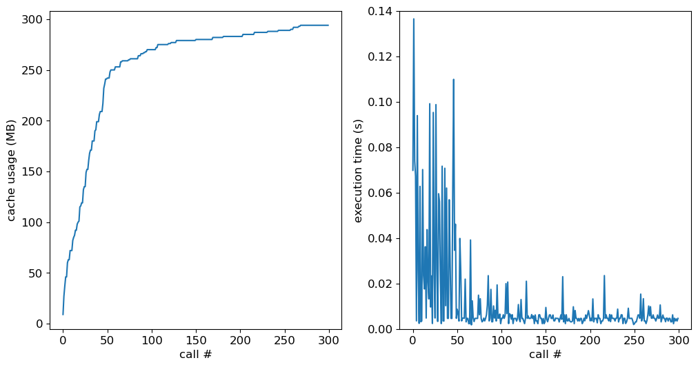
In the left-hand panel we see the cache usage grow and eventually asymptote toward the point where the entire grid (around 400 MB) is resident in memory. In the right-hand panel the execution time rapidly drops from ~0.2s down to ~0.01s, as more and more data can be read from memory (fast) rather than disk (slow).

Let’s now repeat the exercise, but for a cache limit reduced back down to 128 MB:

# Flush the cache and set the limit to 128 MB

specgrid.flush_cache()
specgrid.cache_limit = 128

# Allocate usage & timing arrays

n = 300

cache_usages_128 = np.empty(n, dtype=int)
exec_timings_128 = np.empty(n)

# Call random_flux

for i in range(n):
    exec_timings_128[i] = random_flux()
    cache_usages_128[i] = specgrid.cache_usage

# Plot cache usage and execution time

fig, ax = plt.subplots(ncols=2, figsize=[12,6])

ax[0].plot(cache_usages_512, label='512 MB limit')
ax[0].plot(cache_usages_128, label='128 MB limit')
ax[0].set_xlabel('call #')
ax[0].set_ylabel('cache usage (MB)')
ax[0].legend(loc=4)

ax[1].plot(exec_timings_512)
ax[1].plot(exec_timings_128)
ax[1].set_xlabel('call #')
ax[1].set_ylabel('exution time (s)')

Text(0, 0.5, 'exution time (s)')

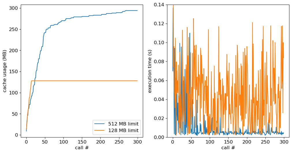
The left-hand panel reveals that, as expected, the growth of the cache usage stops once the limit is reached. Because not all the data can be held in memory, the performance gains from the cache are more modest than in the previous case, with the execution times in the right-hand panel averaging 0.15s.

Choosing Cache Settings

As the demonstration above makes clear, the choice of the pymsg.SpecGrid.cache_usage property can have a significant impact on the performance of MSG. Ideally, this property should be set to exceed the total size of the grid [1]; but if that’s not possible due to limited computer memory, try some of the following measures:

• set the pymsg.SpecGrid.cache_usage property to at least \(4^{N}\) times the size of a single node, where \(N\) is the number of dimensions in a grid (see the Tensor Product Interpolation appendix).

• if undertaking a sequence of interpolations, reorder them so that ones with similar photospheric parameters are grouped together.

• for spectroscopic grids, use the pymsg.SpecGrid.cache_lam_min and/or pymsg.SpecGrid.cache_lam_max properties, as discussed above in the Wavelength Subsetting section.

Technical Details

The basic data unit of MSG’s caches is a grid node, representing the spectroscopic or photometric intensity for a single set of photospheric parameters. During an interpolation the nodes required for the calculation are accessed through the cache, which reads them from disk as necessary. After every node access, the current cache usage is compared against the user-specified limit. If it exceeds this limit, then one or more nodes are evicted from the cache using a least-recently used (LRU) algorithm.

This implementation — with eviction taking place after cache access — means that in principle the cache limit can be zero. For performance reasons, however, this is not recommended.

Footnotes

[1]

Note that the in-memory size of a grid is typically larger than its on-disk size, due to compression.